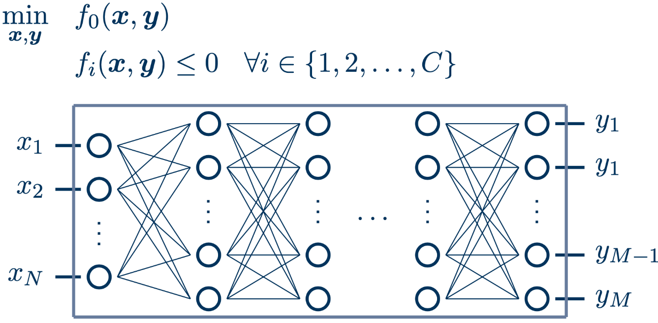
Nonlinear optimization is a critical area in mathematics, dealing with the process of finding the best solution from a set of feasible solutions. Unlike linear optimization, nonlinear optimization involves objective functions or constraints that are nonlinear, making the problem more complex and challenging. In this blog post, we will delve into the key concepts of nonlinear optimization, its mathematical foundations, and its applications.
Nonlinear optimization involves optimizing an objective function subject to constraints, where either the objective function or the constraints (or both) are nonlinear. The general form of a nonlinear optimization problem is:
\[ \min_{x \in \mathbb{R}^n} f(x) \]
subject to:
\[ g_i(x) \leq 0, \quad i = 1, 2, \ldots, m \]
\[ h_j(x) = 0, \quad j = 1, 2, \ldots, p \]
Nonlinear optimization problems can be categorized into several types based on the nature of the objective function and constraints:
The mathematical formulation of a nonlinear optimization problem involves an objective function \( f(x) \) and constraints \( g_i(x) \) and \( h_j(x) \). The problem is to find an optimal solution \( x^* \) that minimizes \( f(x) \) while satisfying all constraints:
\[ \min_{x} f(x) \]
subject to:
\[ g_i(x) \leq 0, \quad i = 1, 2, \ldots, m \]
\[ h_j(x) = 0, \quad j = 1, 2, \ldots, p \]
There are various methods for solving nonlinear optimization problems, each with its own strengths and weaknesses. Some commonly used methods include:
Gradient descent is a simple yet powerful optimization technique. The idea is to iteratively move towards the minimum of the objective function by taking steps proportional to the negative gradient:
\[ x_{k+1} = x_k - \alpha \nabla f(x_k) \]
where \( \alpha \) is the learning rate and \( \nabla f(x_k) \) is the gradient of the objective function at \( x_k \).
Training a neural network involves finding the optimal set of weights that minimize the loss function. This is a nonlinear optimization problem because the loss function is typically nonlinear with respect to the weights. The objective is to minimize the loss function \( L(w) \) with respect to the weights \( w \):
\[ \min_{w} L(w) \]
During training, optimization algorithms like gradient descent are used to update the weights iteratively. The gradients of the loss function with respect to the weights are computed, and the weights are adjusted in the direction that reduces the loss:
\[ w_{k+1} = w_k - \alpha \nabla L(w_k) \]
Here, \( \alpha \) is the learning rate, and \( \nabla L(w_k) \) is the gradient of the loss function at the current set of weights \( w_k \).
Consider a simple neural network with a single hidden layer. The weights between the input layer and the hidden layer are represented as \( W_1 \), and the weights between the hidden layer and the output layer are represented as \( W_2 \). The loss function could be the mean squared error (MSE) between the predicted output and the actual output:
\[ L(W_1, W_2) = \frac{1}{n} \sum_{i=1}^{n} (y_i - \hat{y}_i)^2 \]
where \( y_i \) is the actual output, \( \hat{y}_i \) is the predicted output, and \( n \) is the number of samples. The goal is to minimize \( L(W_1, W_2) \) by adjusting \( W_1 \) and \( W_2 \) using gradient descent.

The MINLP approach
Nonlinear optimization has a wide range of applications in various fields, including:
Nonlinear optimization is a versatile and powerful tool in mathematics, enabling the solution of complex problems across various domains. Understanding the principles and methods of nonlinear optimization is essential for tackling real-world challenges and achieving optimal solutions.
Some Nonlinearity for your linear life: